The following performance numbers are being reported publicly for HANA:
HANA scans data at 3MB/msec/core
On a high-end 80-core server this translates to 240GB/sec per node
HANA inserts rows at 1.5M records/sec/core
Or 120M records/sec per node…
Aggregates 12M records/sec/core
Or 960M records per node…
These numbers seem reasonable:
A 100X improvement over disk-based scan (The recent EMC DCA announcement claimed 2.4GB/sec per node for Greenplum)…
Sort of standard OLTP insert speeds for a big server…
Huge performance gains for in-memory aggregation using columnar orientation and SIMD HPC instructions…
Note that these numbers are the basis for suggesting that there is a new low-TCO approach to BI that eliminates aggregate tables, materialized views, cubes, and indexes… and eliminates the operational overhead of computing these artifacts… and still provides a sub-second response for all queries.
If I were the Register I would have titled this: Raging Stuffed Elephant To Devour Two Warehouse Vendors… I love the Register… if you do not read it have a look…
This is a post is about the market implications of architecture…
Let us assume that Hadoop matures and finds a permanent place in the market. This is not certain with some folks expressing concern (here) and others boundless enthusiasm (here). So let’s assume… and consider where it might fit.
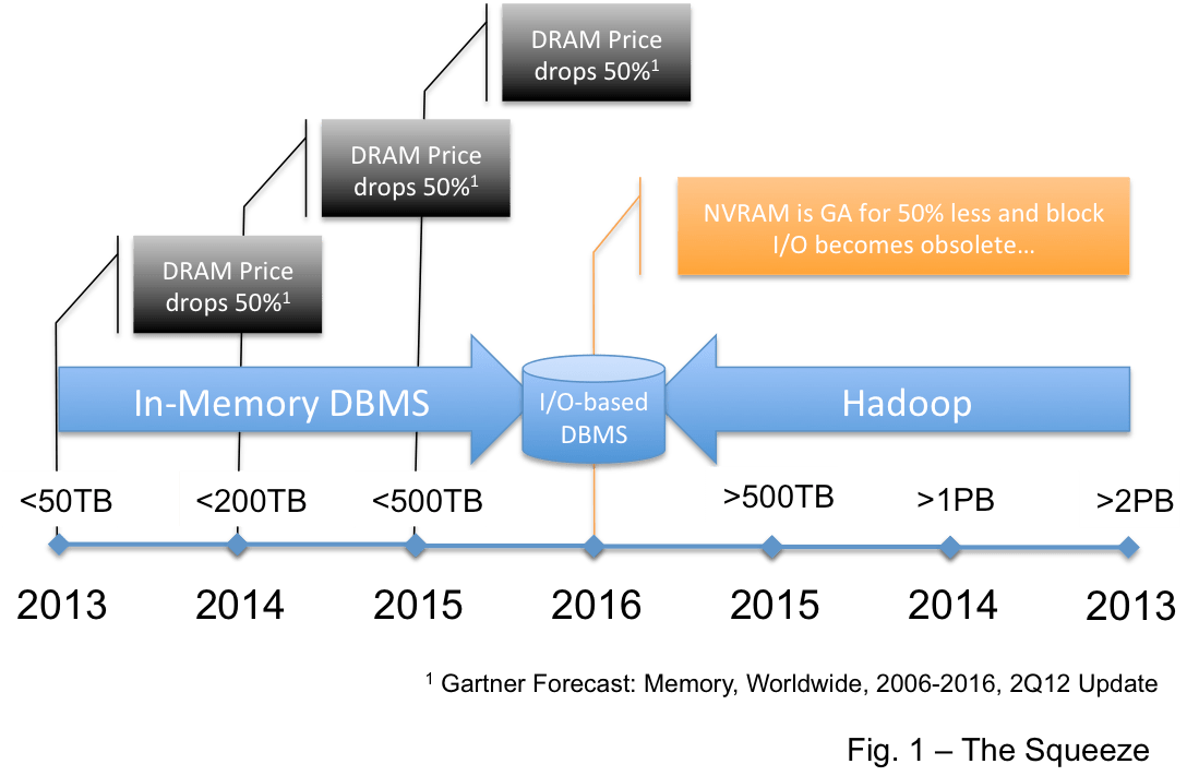
One place is in the data warehouse market… This view says Hadoop replaces the DBMS for data warehouses. But the very mature BI/DW market requires a high level of operational integrity and Hadoop is not there yet… it is advancing rapidly as an enterprise platform and I believe it will get there… but it will be 3-4 years. This is the thinking I provided here that leads me to draw the picture in Figure 1.
It is not that I believe that Hadoop will consume the data warehouse market but I believe that very large EDW’s… those over 1PB… and maybe over 500TB will be compelled by the economics of “free” to move big warehouses to Hadoop. So Hadoop will likely move down into the EDW space from the top.
Another option suggests that Big Data will be a platform unto itself. In this view Hadoop will sit beside the existing BI/DW platform and feed that platform the results of queries that derive structure from unstructured data… and/or that aggregate Big Data into consumable chunks. This is where Hadoop sits today.
In data warehouse terms this positions Hadoop as a very large independent analytic data mart. Figure 2 depicts this. Note that an analytics data mart, and a Hadoop cluster, require far less in the way of operational infrastructure… they share very similar technical requirements.
This leads me to the point of this post… if Hadoop becomes a very large analytic data mart then where will Greenplum and Netezza fit in 2-3 years? Both vendors are positioning themselves in the analytic space… Greenplum almost exclusively so. Both vendors offer integrated Hadoop products… Greenplum offers the Greenplum database and Hadoop in the same hardware cluster (see here for their latest announcement)… Netezza provides a Hadoop connector (here). But if you believe in Hadoop… as both vendors ardently do… where do their databases fit in the analytics space once Hadoop matures and fully supports SQL? In the next 3-4 years what will these RDBMSs offer in the big data analytics space that will be compelling enough to make the configuration in Figure 3 attractive?
I know that today Hadoop cannot do all that either Netezza or Greenplum can do. I understand that Netezza has two positions in the market… as an analytic appliance and as a data mart appliance… so it may survive in the mart space. But the overlap of technical requirements between Hadoop and an analytic data mart… combined with the enormous human investment in Hadoop R&D, both in the core and in the eco-system… make me wonder about where “Big Data” analytic relational databases will fit?
Note that this is not a criticism of the Greenplum RDBMS. Greenplum is a very fine product, one of the best EDW platforms around. I’ll have more to say about it when I provide my 2 Cents… But if Figure 2 describes the end state for analytics in 2-3 years then where is the place for the Figure 3 architecture? If Figure 3 is the end state then I do not see where the line will be drawn between the analytic workload that requires Greenplum and that that will run on Hadoop? I barely can see it now… and I cannot see it at all in the near future.
Both EMC Greenplum and IBM seem to strongly believe in Hadoop… they must see the overlap in functionality and feel the market momentum of Hadoop. They must see, better than most, that Hadoop wins this battle.
This post has been thrown at me a couple of times now… so I’ll now take the time to go through it… and try to address the junk.
It starts by suggesting that “the Germans” have started a war… but the next sentence points out that the author tossed grenades at HANA two months before the start he suggests. It also ignores the fact that the HANA post in question was a response to incorrect public statements by a Microsoft product manager about HANA (here).
The author suggests some issue with understanding clustered indexes… Note that “There are 2 implementations of xVelocity columnstore technology: 1. Non clustered index which is read only – this is the version available in SMP (single node) SQL Server 2012. 2. Columnstore as a clustered index that is updateable – This is the version available in MPP or PDW version of SQL 2012.”. The Microsoft documentation I read did not distinguish between the two and so I mistakenly attributed features of one to the other. Hopefully this clears up the confusion.
He suggests that the concept of keeping redundant versions of the data… one for OLTP and one for BI is “untrue”… I believe that the conventional way to deal with OLTP and BI is to build separate OLTP and BI databases… data warehouses and data marts. So I stand by the original comment.
The author rightfully suggests that I did not provide a reference for my claim that there are odd limitations to the SQL that require hand-coding… here they are (see the do’s and dont’s).
He criticizes my statement that shared-nothing gave us the basis for solving “big data”. I do not understand the criticism? Nearly very large database in the world is based on a shared-nothing architecture… and the SQL Server PDW is based on the same architecture in order to allow SQL Server to scale.
He is critical of the fact that HANA is optimized for the hardware and suggests that HANA does not support Intel’s Ivy Bridge. HANA is optimized for Ivy Bridge… and HANA is designed to fully utilize the hardware… If we keep it simple and suggest that using hardware-specific instruction sets and hardware-specific techniques to keep data in cache together provide a 50X performance boost [This ignores the advantages of in-memory and focusses only on hw-specific optimizations… where data in cache is either 15X (L3) or 20X (L2) or 200X (L1) faster than data fetched from DRAM… plus 10X or more using super-computer SIMD instructions], I would ask… would you spend 50X more for under-utilized hardware if you had a choice? SAP is pursuing a distinct strategy that deserves a more thoughtful response than the author provided.
He accuses me of lying… lying… about SQL being architected for single-core x286 processors. Sigh. I am unaware of a rewrite of the SQL Server product since the 286… and tacking on support for modern processors is not re-architecting. If SQL Server was re-architected from scratch since then I would be happy to know that I was mistaken… but until I hear about a re-write I will assume the SQL Server architecture, the architecture, is unchanged from when Sybase originally developed it and licensed it to Microsoft.
He says that HANA is cobbled together from older piece parts… and points to a Wikipedia page. But he does not use the words in the article… that HANA was synthesized from other products and , as stated in the next sentence, built on: “a new application architecture“. So he leaves the reader to believe that there is nothing new… he is mistaken. HANA is more than a synthesis of in-memory, column-store, and shared-nothing. It includes a new execution engine built on algorithms from the search space… columns in the column store are processed as vectors rather than the rote tuple-by-tuple approach from the 1980’s. It includes powerful in-database support for procedural languages with facilities that convert loops to fully parallel set-based processes. It provides, as noted above, a unique approach to supporting OLTP and BI queries in the same instance (see here)… and more. I’m not trying to hype HANA here… time and the market will determine if these new features are important… but there is no doubt that they are new.
I did not find the Business Intelligist post to be very informative or helpful. With the exception of the Wikipedia article mentioned above there is only unsubstantiated opinion in the piece… … and a degree of rudeness that is wholly uncalled for.
Aerial view of Hana, Maui (Photo credit: Wikipedia)
This is a rehash of my post for SAP here… I thought you might find it interesting as it describes the architecture HANA uses to support OLTP and BI against a single table.
A couple of points to think about:
If you have only one database structure you can optimize for only one query; e.g. the OLTP query is fast against a OLTP structure but slow against a BI structure… or visa versa.
If you have two structures you have to ETL the data between the two at some cost. There is cost in keeping a replica of the data, cost in developing, administering, and executing the ETL process. In addition there is a lost opportunity cost hidden in the latency of the data. You cannot see the current state of the business by querying the BI data as some data has not yet been ETL’d across.
OLTP performance is normally paramount; so the perfect system would not compromise that performance or compromise it only a little.
Let’s look at the HANA approach to this at a high level.
HANA provides a single view of a table to an application or a user, but under-the-covers each table includes a OLTP optimized part, a BI optimized part, and a mechanism for moving data from one part to the other
When a transaction hits the system; inserts, updates, and deletes are processed in the OLTP part with no performance penalty. The read portion of the OLTP query accesses the read-optimized internal structure with no performance penalty. Note that reading a single column in a column store, which is the key for the transaction, is roughly equivalent to reading an index structure on top of a standard disk-based DBMS. Except the column is always in-memory which means I/O is never required. This provides the HANA system with an advantage over a disk-based system. Disk I/O is 120+ times slower than memory access so even an index is unlikely to beat in-memory. See here for some numbers you should know.
After the transaction is committed into the internal, OLTP-optimized part, a process starts that moves the data to the BI optimized part. This is called a delta merge as the OLTP portion holds all of the changes, the delta, in the data set.
When a BI query starts it can limit the scan to only partitions in the BI optimized part, or if real-time data is required it can scan both parts. The small portion of the scan that accesses the OLTP/delta portion is sub-optimal when compared to the scan of the BI part, but not slow at all as the data is all in-memory.
We can tease the performance apart as follows:
There is a OLTP insert/update/delete “write” portion… and HANA executes this like any OLTP database, as fast as an OLTP RDBMS, with a commit after a write-to-log;
There is a OLTP select “read” portion… and HANA performs this in the in-memory column store faster than many OLTP databases… and scans the delta structure as fast as any OLTP database;
There is a delta merge from the OLTP write-optimized part to the BI read-optimized column store that is hundreds to tens of thousands of times faster than any ETL tool; and
There is a BI select portion that scans the in-memory column store hundreds to thousands of times faster than a disk-based BI database.
If the BI query requires access to real-time data then an in-memory scan of the delta file is required… there is no analogy to this in a system with separate OLTP and BI tables.
There seems to be a sort of odd tradition for bloggers to look back at the past year as the New Year starts to unfold. Here is my review of my posts and some presents
(Photo credit: Wikipedia)
…
Top Post
Far and away the most viewed post was Exalytics vs. HANA What are they thinking? This simply notes that these two products are not really comparable sharing only the descriptor “in-memory”.
These papers and the underlying thinking by smarter folks than I will inform you about the definition of Hot Data from the point of pure IT economics.
The Most Under-rated Post
This is the post I thought was the most important… as it might strongly influence data warehouse platform buying decisions over the next few years… And it might even influence the stocks you pick: The Future of Hadoop and Big Data DBMSs
Some Other Posts to Read
Here are two posts that informed me:
The Five Minute Rule… This will point you to a Wikipedia article that will point you to the whole series of papers.
What Every Programmer Should Know About Memory… This paper goes into gory detail about how memory works inside a processor. It is hardware-centric for you software folks… but provides the basis for understanding why in-memory DBMSs are fast and why Exadata is not an in-memory DBMS.
I posted a blog on the SAP site here that discussed the implications of mobile clients. I want to re-emphasize the issue as it is crucial.
While at Greenplum we routinely replaced older EDW platforms and provided stunning performance. I recall one customer in particular where we were given a query that ran in 7 hours and Greenplum executed the query in seven seconds. This was exceptional… more typical were cases where we reduced run-times from several hours to under 30 minutes… to 10 minutes… to 5 minutes. I’m sure that every major competitor: Teradata, Greenplum, Netezza, and Exadata has similar stories to tell.
But 5 minutes will not cut it if you are servicing a mobile client where sub-second response to the device is a requirement… and 10 minutes is out of the question. It does not matter if it ran in 10 hours before… 10 minute response is not acceptable to a mobile device.
Today we see sub-second response delivered to our phones by custom applications built on special high-performance platforms designed specifically to service a mobile client: iPhones, iPads, and Android devices.
But what will we do about the BI applications built on commercial platforms which have just used every trick in the book to become one of the 5 minute stories mentioned above?
I think that there are only a couple of architectural choices.
We can rewrite the high-value queries as custom applications using specialized infrastructure… at great expense… and leaving the vast majority of queries un-serviced.
We can apply the 80/20 rule to get the easiest queries serviced with only 20% of the effort. But according to Murphy the 20% left will be the highest value queries.
We can tack on expensive, specialized, accelerators to some queries… to those that can be accelerated… but again we leave too much behind.
Or we can move to a general purpose high performance computing platform that can service the existing BI workload with sub-second response.
In-memory computing will play a role… Exalytics provides option #3… HANA option #4.
SSD devices may play a role… but the performance improvements being quoted by vendors who use SSD as a block I/O device is 10X or less. A 10X improvement applied to a query that was just improved to 10 minutes yields a 1 minute query… still not the expected level of service.
IT departments will have to evaluate the price/performance, not just the price, as they consider their next platform purchases. The definition of adequate response is changing… and the old adequate, at the least cost, may not cut it. Mobile clients are here to stay. The productivity gains expected from these devices is significant. High performance BI computing is going to be a requirement.
When I was at Greenplum… and now again at SAP… I ran into a strange logic from Teradata about query concurrency. They claimed that query concurrency was a good thing and an indicator of excellent workload management. Let’s look at a simple picture of how that works.
In Figure 1 we depict a single query on a Teradata cluster. Since each node is working in parallel the picture is representative no matter how many nodes are attached. In the picture each line represents the time it takes to read a block from disk. To make the picture simple we will show I/O taking only 1/10th of the clock time… in the real world it is slower.
Given this simplification we can see that a single query can only consume 10% of the CPU… and the rest of the time the CPU is idle… waiting for work. We also represented some I/O to spool files… as Teradata writes all intermediate results to disk and then reads them in the next step. But this picture is a little unfair to Greenplum and HANA as I do not represent spool I/O completely. For each qualifying row the data is read from the table on disk, written to spool, and then read from spool in the subsequent step. But this note is about concurrency… so I simplified the picture.
Figure 2 shows the same query running on Greenplum. Note that Greenplum uses a data flow architecture that pushes tuples from step to step in the execution plan without writing them to disk. As a result the query completes very quickly after the last tuple is scanned from the table.
Let me say again… this story is about CPU utilization, concurrency, and workload management… I’m not trying to say that there are not optimizations that might make Teradata outperform Greenplum… or optimizations that might make Greenplum even faster still… I just want you to see the impact on concurrency of the spool architecture versus the data flow architecture.
Note that on Greenplum the processors are 20% busy in the interval that the query runs. For complex queries with lots of steps the data flow architecture provides an even more significant advantage to Greenplum. If there are 20 steps in the execution plan then Teradata will do spool I/O, first writing then reading the intermediate results while Greenplum manages all of the results in-memory after the initial reads.
In Figure 3 we see the impact of having the data in-memory as with HANA or TimeTen. Again, I am ignoring the implications of HANA’s columnar orientation and so forth… but you can clearly see the implications by removing block I/O.
Now let’s look at the same pictures with 2 concurrent queries. Let’s assume no workload management… just first in, first out.
In Figure 4 we see Teradata with two concurrent queries. Teradata has both queries executing at the same time. The second query is using up the wasted space made available while the CPUs wait for Query 1’s I/O to complete. Teradata spools the intermediate results to disk; which reduces the impact on memory while they wait. This is very wasteful as described here and here (in short, the Five Minute Rule suggests that data that will be reused right away is more economically stored in memory)… but Teradata carries a legacy from the days when memory was dear.
But to be sure… Teradata has two queries running concurrently. And the CPU is now 20% busy.
Figure 5 shows the two-query picture for Greenplum. Like Teradata, they use the gaps to do work and get both queries running concurrently. Greenplum uses the CPU much more efficiently and does not write and read to spool in between every step.
In Figure 6 we see HANA with two queries. Since one query consumed all of the CPU the second query waits… then blasts through. There is no concurrency… but the work is completed in a fraction of the time required by Teradata.
If we continue to add queries using these simple models we would get to the point where there is no CPU available on any architecture. At this point workload management comes into play. If there is no CPU then all that can be done is to either manage queries in a queue… letting them wait for resources to start… or start them and let them wastefully thrash in and out… there is really no other architectural option.
So using this very simple depiction eventually all three systems find themselves in the same spot… no CPU to spare. But there is much more to the topic and I’ve hinted about these in previous posts.
Starting more queries than you can service is wasteful. Queries have to swap in and out of memory and/or in and out of spool (more I/O!) and/or in and out of the processor caches. It is best to control concurrency… not embrace it.
Running virtual instances of the database instead of lightweight threads adds significant communications overhead. Instances often become unbalanced as the data returned makes the shards uneven. Since queries end when the slowest instance finishes it’s work this can reduce query performance. Each time you preempt a running query you have to restore state and repopulate the processor’s cache… which slows the query by 12X-20X. … Columnar storage helps… but if the data is decompressed too soon then the help is sub-optimal… and so on… all of the tricks used by databases and described in these blogs count.
But what does not count is query concurrency. When Teradata plays this card against Greenplum or HANA they are not talking architecture… it is silliness. Query throughput is what matters. Anyone would take a system that processes 100,000 queries per hour over a system that processes 50,000 queries per hour but lets them all run concurrently.
I’ve been picking on Teradata lately as they have been marketing hard… a little too hard. Teradata is a fine system and they should be proud of their architecture and their place in the market. I am proud to have worked for them. I’ll lay off for a while.
I recently pointed out some silliness published by Teradata to several SAP prospects. There is more nonsense that was sent and I’d like to take a moment to clear up these additional claims.
In their note to HANA prospects they used the following numbers from the paper SAP published here:
Teradata makes several claims from these numbers. First they claim that the numbers demonstrate a bottleneck that is tied to either the NUMA effect or to the SMP Knee Curve. This nonsense is the subject of a previous blog here.
For any database system as you increase the number of queries to the point where there is contention the throughput decreases. This is just common sense. If you have 10 cores and 10 threads and there is no contention then all threads run at the same speed as fast as possible. If you add an 11th thread then throughput falls off, as one thread has to wait for a core. As you add more threads the throughput falls further until the system is saturated and throughput flattens. Figure 1 is an example of the saturation curve you would expect from any system as the throughput flattens.
There are some funny twists to this, though. If you are an IMDB then each query can use 100% of a core. If you are multi-threaded IMDB then each query can use 100% of all cores. If you are a disk-based system then you give up the CPU to another query while you wait for I/O… so throughput falls. I’ll address these twists in a separate blog… but you will see a hint at the issue here.
Teradata claims that these numbers reflect a scaling issue. This is a very strange claim. Teradata tests scaling by adding hardware, data, and queries in equal amounts to see if the query performance holds constant… or they add hardware and data to look for a correlation between the number of nodes and query performance… hoping that as the nodes increase the response time decreases. In fact Teradata scales well… as does HANA… But the hardware is constant in the HANA benchmark so there is no view into scaling at all. Let me emphasis this… you cannot say anything about scaling from the numbers above.
Teradata claims that they can extrapolate the saturation point for the system… this represents very bad mathematics. They take the four data points in the table and create an S curve like the one in Figure 1… except they invert it to show how throughput decreases as you move towards the saturation point… Figure 2 shows the problem.
If you draw a straight line through the curve using any sort of math you miss the long tail at the end. This is an approximation of the picture Teradata drew… but even in their picture you can see a tail forming… which they ignore. It is also questionable math to extrapolate from only four observations. The bottom line is that you cannot extrapolate the saturation point from these four numbers… you just don’t know how far out the tail will run unless you measure it.
To prove this is nonsense you just have to look here. It turns out that SAP publicly published these benchmark results in two separate papers and this second one has numbers out to 60 streams. Unsurprisingly at 60 streams HANA processed 112,602 queries per hour while Teradata told their customers that it would saturate well short of that… at 49,601 queries (they predicted that HANA would thrash and the number of queries/hour would fall back… more FUD).
Teradata is sending propaganda to their prospects with scary extrapolations and pronouncements of architectural bottlenecks in HANA. The mathematics behind their numbers is weak and their incorrect use of deep architectural terms demonstrates ignorance of the concepts. They are trying to create Fear, Uncertainty, and Doubt. Bad marketing… not architecture, methinks.
Here is one I composed for SAP on the HANA blog about the recent Microsoft SQL Server announcements that is not too obnoxiously pro-HANA. It is more about the data architecture required to handle a world where the client is a mobile device and every query must complete sub-second. This, I believe is where we are headed… taking those BI queries that run in an hour on weak warehouses and improving the response to 10 seconds won’t cut it if your user is on a mobile device… and if the query is customer-facing you will be out of business…
The only way to solve for this is to get lots of silicon between you and your data… and hope that no queries miss the cache… or put it all in-memory.
———
I might have added to the work post that anytime a database vendor pre-announces a product that is due out in 1-2 years, “2014-2015” in this case, it is marketing not architecture… meant to freeze SQL Server customers in place while Microsoft tries to catch up.
Make sure to have a look at the comments… there is a great link to a Microsoft mouthpiece who suggests that I must have no technical background and that I am a liar. Nice.
Teradata is circulating a document to customers that claims that the numbers SAP has published in its 100TB PoC white paper (here) demonstrates that HANA suffers from scaling issues associated with the NUMA-effect. The document is so annoyingly inaccurate that I have to respond.
NUMA stands for non-uniform-memory-access. This describes an architecture whereby each core in a multi-core system has some very fast local memory accessed directly through a memory bus… but has access to every other core’s local memory through a “remote” access hop over another fast bus. In the case of Intel Xeon servers the other fast bus is know as the QPI bus. “Non-uniform” means that all memory access are not equal… a remote access over the QPI bus is slower than access over the memory bus.
The first mistake in the Teradata document is where they refer to the problem as the “SMP Knee Curve”. SMP stands for symmetric multi-processing… an architecture where multiple cores share the same memory bus. The SMP Knee Curve describes the problem when too many cores are contending for the same bus. HANA is not certified to run on an SMP system. The 100TB PoC described above is not run on an SMP system. When describing issues you might expect Teradata to at least associate the issue with the correct hardware architecture.
The NUMA-effect describes problems scaling processors within a single NUMA node. Those issues can impact the ability to continuously add cores as memory locking issues across the QPI bus slow the system. There are ways to mitigate this problem, though (see here for some examples of how to code around the problem).
Of course HANA, which built an in-memory system with NUMA as a target from the start… has built in these NUMA mitigations. In fact, HANA is designed deeper still using special techniques to keep the processor caches filled and to invoke special-purpose SIMD instructions. HANA is built so close to the hardware that processor cycles that are unused due to cache misses but show up as processor busy are avoided (in other words, HANA will get more work done on a 100% CPU busy system than other software that will show 100% CPU busy). But Teradata chose to ignore this deep integration… or they were unaware of these techniques.
Worse still, the problem Teradata calls out… shouts out… is about scaling over 100 nodes in a shared-nothing configuration. The NUMA-effect has nothing at all to do with scale out across nodes. It is an issue within a single node. For Teradata to claim this is silliness at best. It is especially silly since the shared-nothing architecture upon which HANA is built is the same architecture Teradata uses.
The twists Teradata applies to the numbers are equally absurd… but I’ll stop here and hope that the lack of understanding they exhibit in throwing around terms like “SMP Knee Curve” and “NUMA-effect” will cast enough doubt that the rest of their marketing FUD will be suspect. Their document is surely not about architecture… it is weak marketing… you can see more here…